Instructions
Requirements and Specifications


Source Code
CODE 1
# -*- coding: utf-8 -*-
"""Question1.ipynb
Automatically generated by Colaboratory.
Original file is located at
https://colab.research.google.com/drive/1aNZzpp0PCP_IW3AyUhYQLspE1Sb9wSRz
"""
import numpy as np
import pandas as pd
import matplotlib.pyplot as plt
from sklearn.model_selection import StratifiedKFold
import tensorflow as tf
from sklearn.preprocessing import MinMaxScaler
from sklearn.preprocessing import LabelBinarizer
"""# Question 1
We will use a model to do a Logistic Regression in order to predit TA Performance
### Read Data
"""
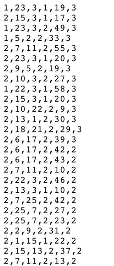
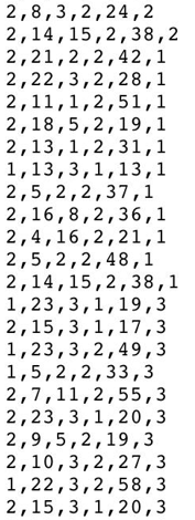
df = pd.read_csv("TA_evals.txt", names = ["English Speaker", "Instructor", "Course", "Summer", "Class Size", "TA Performance"])
df.head()
df_original = df.copy()
"""### Get dummies for categorical columns"""
columns = ["Instructor", "Course"]
for column in columns:
df = pd.concat([df, pd.get_dummies(df[column], prefix=column)], axis=1)
df = df.drop(column, axis=1)
df.head()
"""### Normalize Class Size"""
scaler = MinMaxScaler()
df["Class Size"] = scaler.fit_transform(df["Class Size"].values.reshape(-1,1))
"""### Binarize 'English Speaker' and 'Summer'"""
lb = LabelBinarizer()
df["English Speaker"] = lb.fit_transform(df["English Speaker"].values.reshape(-1,1))
df["Summer"] = lb.fit_transform(df["Summer"].values.reshape(-1,1))
"""### Convert 'TA Performance' to zero indexing"""
df["TA Performance"] -= 1
df.head()
"""### Split data into X and y"""
y = df["TA Performance"].values
X = df.drop(columns=["TA Performance"]).values
"""# Model 1: Sequential model with 3 Dense layers and Adam Optimizer"""
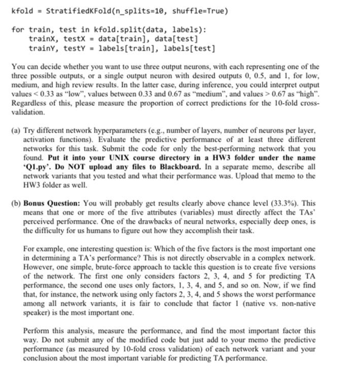
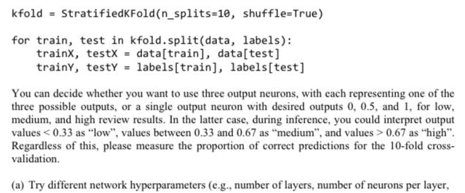
kfold = StratifiedKFold(n_splits=10, shuffle=True)
fig, axes = plt.subplots(nrows = 1, ncols = 2)
for train, test in kfold.split(X, y):
trainX, testX = X[train], X[test]
trainY, testY = y[train], y[test]
# For each dataset, create a model
model = tf.keras.models.Sequential()
model.add(tf.keras.layers.Dense(32, activation='relu', input_dim=trainX.shape[1]))
model.add(tf.keras.layers.Dense(64, activation='relu'))
model.add(tf.keras.layers.Dense(3, activation='softmax'))
model.compile(optimizer='adam', loss = 'sparse_categorical_crossentropy', metrics=['acc'])
history = model.fit(trainX, trainY, epochs= 500, verbose=0)
axes[0].plot(history.history['acc'])
axes[1].plot(history.history['loss'])
axes[0].set_xlabel('Epochs')
axes[0].set_title('Accuracy')
axes[1].set_xlabel('Epochs')
axes[1].set_title('Loss')
plt.show()
"""# Model 2: Sequential model with 3 Dense layer, 1 BatchNormalization layer and Number of neurons doubled"""
fig, axes = plt.subplots(nrows = 1, ncols = 2)
for train, test in kfold.split(X, y):
trainX, testX = X[train], X[test]
trainY, testY = y[train], y[test]
# For each dataset, create a model
model = tf.keras.models.Sequential()
model.add(tf.keras.layers.Dense(64, activation='relu', input_dim=trainX.shape[1]))
model.add(tf.keras.layers.Dense(128, activation='relu'))
model.add(tf.keras.layers.BatchNormalization(trainable=True))
model.add(tf.keras.layers.Dense(3, activation='softmax'))
model.compile(optimizer='adam', loss = 'sparse_categorical_crossentropy', metrics=['acc'])
history = model.fit(trainX, trainY, epochs= 500, verbose=0)
axes[0].plot(history.history['acc'])
axes[1].plot(history.history['loss'])
axes[0].set_xlabel('Epochs')
axes[0].set_title('Accuracy')
axes[1].set_xlabel('Epochs')
axes[1].set_title('Loss')
plt.show()
"""# Model 3: Model with 4 Dense layers,Stochastic Gradient Descend and Sigmoid activation on output layer"""
fig, axes = plt.subplots(nrows = 1, ncols = 2)
for train, test in kfold.split(X, y):
trainX, testX = X[train], X[test]
trainY, testY = y[train], y[test]
# For each dataset, create a model
model = tf.keras.models.Sequential()
model.add(tf.keras.layers.Dense(trainX.shape[1], activation='relu', input_dim=trainX.shape[1]))
model.add(tf.keras.layers.Dense(32, activation='relu'))
model.add(tf.keras.layers.Dense(64, activation='relu'))
model.add(tf.keras.layers.Dense(128, activation='relu'))
model.add(tf.keras.layers.Dense(256, activation='relu'))
model.add(tf.keras.layers.Dense(3, activation='sigmoid'))
model.compile(optimizer='sgd', loss = 'sparse_categorical_crossentropy', metrics=['acc'])
history = model.fit(trainX, trainY, epochs= 500, verbose=0)
axes[0].plot(history.history['acc'])
axes[1].plot(history.history['loss'])
axes[0].set_xlabel('Epochs')
axes[0].set_title('Accuracy')
axes[1].set_xlabel('Epochs')
axes[1].set_title('Loss')
plt.show()
"""# Model 4: Model 1 but increasing epochs and number of neurons"""
fig, axes = plt.subplots(nrows = 1, ncols = 2)
for train, test in kfold.split(X, y):
trainX, testX = X[train], X[test]
trainY, testY = y[train], y[test]
# For each dataset, create a model
model = tf.keras.models.Sequential()
model.add(tf.keras.layers.Dense(trainX.shape[1], activation='relu', input_dim=trainX.shape[1]))
model.add(tf.keras.layers.Dense(16, activation='relu'))
model.add(tf.keras.layers.Dense(3, activation='softmax'))
model.compile(optimizer='adam', loss = 'sparse_categorical_crossentropy', metrics=['acc'])
history = model.fit(trainX, trainY, epochs= 1000, verbose=0)
axes[0].plot(history.history['acc'])
axes[1].plot(history.history['loss'])
axes[0].set_xlabel('Epochs')
axes[0].set_title('Accuracy')
axes[1].set_xlabel('Epochs')
axes[1].set_title('Loss')
plt.show()
"""We tried different variations of the model as can be seen above, with models 1, 2, 3 and 4. Apart from these 4 models, I also played with the activation functions (SGD, RMSprop, Adam, etc) and different number of layers, number of neurons, etc. However, the best model was still Model 1 (which is very simple but returned the best accuracy/loss curves without oscillations).
# Part b) We will test the model from previous part with the highest accuracy. We will remove one feature from data at time, and run the model 10 that data
"""
# We take the original dataset
features = [x for x in df_original.columns if x != 'TA Performance']
n_features = len(features)
# Create a figure with n_features rows showing the model with each feature removed
fig, axes = plt.subplots(nrows = n_features, ncols = 2, figsize=(25,25))
# Kfold
kfold = StratifiedKFold(n_splits=10, shuffle=True)
# Now, start removing one feature at the time
fig_id = 0
for ft in features:
df = df_original.copy()
# Normalize class size
scaler = MinMaxScaler()
df["Class Size"] = scaler.fit_transform(df["Class Size"].values.reshape(-1,1))
# Binarize 'English Speaker' and 'Summer'
lb = LabelBinarizer()
df["English Speaker"] = lb.fit_transform(df["English Speaker"].values.reshape(-1,1))
df["Summer"] = lb.fit_transform(df["Summer"].values.reshape(-1,1))
# Convert the y variable to zero-indexing
df["TA Performance"] -= 1
df = df.drop(columns=[ft], axis=1)
# Now, if Instructor and Course are still in the dataset, get dummies
columns = ["Instructor", "Course"]
for column in columns:
if column in df.columns:
df = pd.concat([df, pd.get_dummies(df[column], prefix=column)], axis=1)
df = df.drop(column, axis=1)
# Splot into X and y
y = df["TA Performance"].values
X = df.drop(columns=["TA Performance"]).values
# Now, run models
for train, test in kfold.split(X, y):
trainX, testX = X[train], X[test]
trainY, testY = y[train], y[test]
# For each dataset, create a model
model = tf.keras.models.Sequential()
model.add(tf.keras.layers.Dense(32, activation='relu', input_dim=trainX.shape[1]))
model.add(tf.keras.layers.Dense(64, activation='relu'))
model.add(tf.keras.layers.Dense(3, activation='softmax'))
model.compile(optimizer='adam', loss = 'sparse_categorical_crossentropy', metrics=['acc'])
history = model.fit(trainX, trainY, epochs= 500, verbose=0)
axes[fig_id, 0].plot(history.history['acc'])
axes[fig_id, 1].plot(history.history['loss'])
axes[fig_id, 0].set_title(ft)
fig_id += 1
plt.show()
"""From curves above, it can be seen that the best accuracy curves were obtained when we removed the 'Summer' feature. This means that, if the course is a Summer course or not, it does not affects the TA Performance at all."""
CODE 2
# -*- coding: utf-8 -*-
"""Question2.ipynb
Automatically generated by Colaboratory.
Original file is located at
https://colab.research.google.com/drive/1jPj8WPPQQwjIN85yqgE-2L5R9S3QD8bI
"""
import numpy as np
import pandas as pd
import matplotlib.pyplot as plt
import cv2
from sklearn.model_selection import train_test_split
import tensorflow as tf
"""# Download Dataset"""
!gdown --id 1psl9Ok84KuZDOPQibtfNSustu-q5dG7p
!gdown --id 1Nn95-vjPjxN88cHvu8J5bIzj6HSqgDHo
"""# Load"""
x = np.load('batch_00.npz')['arr_0']
y = np.load('batch_00_labels.npz')['arr_0']
# To reduce the time the model takes to run, we will use only the first 5000 images
#x = x[:5000]
#y = y[:5000]
x_rescaled = np.zeros((len(x), 28, 28))
for i in range(len(x)):
x_rescaled[i] = cv2.resize(x[i], (28,28), interpolation = cv2.INTER_CUBIC)
x_train, x_test, y_train, y_test = train_test_split(x_rescaled, y, test_size = 0.2)
x_train = np.expand_dims(x_train, 3)
x_test = np.expand_dims(x_test, 3)
# Normalize
x_train, x_test = x_train/255.0, x_test/255.0
n_labels = len(np.unique(y))
"""# Create Model"""
model = tf.keras.Sequential([
tf.keras.layers.Conv2D(16, (3,3), input_shape = (28,28,1), activation = 'relu'),
tf.keras.layers.MaxPooling2D(2,2),
tf.keras.layers.Dropout(0.05),
tf.keras.layers.Conv2D(32, (3,3), activation = 'relu'),
tf.keras.layers.MaxPooling2D(2,2),
tf.keras.layers.Dropout(0.05),
tf.keras.layers.Conv2D(64, (3,3), activation = 'relu'),
tf.keras.layers.MaxPooling2D(2,2),
tf.keras.layers.Flatten(),
tf.keras.layers.Dense(512, activation = 'relu'),
tf.keras.layers.Dense(n_labels, activation = 'softmax')])
model.summary()
model.compile(optimizer = 'adam', loss = 'sparse_categorical_crossentropy', metrics = ['accuracy'])
history = model.fit(x_train, y_train, epochs = 50, validation_data = (x_test, y_test))
plt.figure()
plt.plot(history.history['accuracy'], label='Accuracy')
plt.plot(history.history['loss'], label = 'Loss')
plt.plot(history.history['val_accuracy'], label = 'Val Accuracy')
plt.plot(history.history['val_loss'], label = 'Val Loss')
plt.xlabel('Epochs')
plt.legend()
plt.grid(True)
plt.show()
"""The model presented above is the model with the best performance. I've tried different variations, adding more Convolutional Layers, changing the size of the filters, adding Dropout, changing activation function, optimizers, but in the end, the best performance i the one shown. For all other model, the Validation Loss started to increase after ~30 EPOCHS, the accuracy was below 70%, etc.
# Part b) Model without Convolutional Layers
"""
model = tf.keras.Sequential([
tf.keras.layers.Dense(32, input_shape = (28,28,1)),
tf.keras.layers.Dense(32, activation='relu'),
tf.keras.layers.Dense(64, activation = 'relu'),
tf.keras.layers.Flatten(),
tf.keras.layers.Dense(n_labels, activation = 'softmax')])
model.compile(optimizer = 'adam', loss = 'sparse_categorical_crossentropy', metrics = ['accuracy'])
history = model.fit(x_train, y_train, epochs = 50, validation_data = (x_test, y_test))
plt.figure()
plt.plot(history.history['accuracy'], label='Accuracy')
plt.plot(history.history['loss'], label = 'Loss')
plt.plot(history.history['val_accuracy'], label = 'Val Accuracy')
plt.plot(history.history['val_loss'], label = 'Val Loss')
plt.xlabel('Epochs')
plt.legend()
plt.grid(True)
plt.show()
"""For this case, we removed all convoltional Layers and used only Dense layers. The model response was good for a small amount of data (~5000 images), however, the model is over-fitted as the Accuracy reaches 1.0.
However, we could not test the model with all the dataset because it just takes too much time to run (approx 20min per epoch)
"""