Instructions
Requirements and Specifications
Source Code
import matplotlib.pyplot as plt
import seaborn as sns
from sympy import *
import urllib.request
import random
from sympy.plotting.plot import Plot, ContourSeries
import numpy as np
def Problem1():
print("Running problem 1...")
# Create the symbolic variable x
x = Symbol('x')
# Create function
f = 10 - 4 * x ** 2 + 2 * x ** 3
# Get its minimum
fprime = f.diff(x)
x_min = solve(fprime, x)[1]
f_xmin = f.subs(x, x_min)
# Plot
#plot(f, (x, 0, 8 / 4), xlim=(0, 8 / 4), ylim=(30 / 4, 40 / 4), xlabel='X', ylabel='Y', label='Function', show = False)
xvals = np.linspace(0, 8/4, 100)
fvals = lambdify(x, f)(xvals)
plt.figure()
plt.plot(xvals, fvals, label = f)
plt.plot(x_min, f_xmin,'r*', label = 'Local Minimum')
plt.xlim([0, 8/4])
plt.ylim([30/4, 40/4])
plt.xlabel('X')
plt.ylabel('Y')
plt.legend()
plt.xticks([0, 1/4, 2/4, 3/4, 4/4, 5/4, 6/4, 7/4, 8/4], ['0', '1/4', '2/4', '3/4', '4/4', '5/4', '6/4', '7/4', '8/4'])
plt.yticks([30/4, 32/4, 34/4, 36/4, 38/4, 40/4], ['30/4', '32/4', '34/4', '36/4', '38/4', '40/4'])
plt.show()
"""plt.xticks(['0', '1/4', '2/4', '3/4', '4/4', '5/4', '6/4', '7/4', '8/4'])
plt.yticks([30/4, 31/4, 32/4, 33/4, 34/4, 35/4, 36/4, 37/4, 38/4, 39/4, 40/4])
plt.label()
plt.show()"""
def Problem2():
print("Running Problem 2...")
# Define alpha and beta
alpha = 0.5
beta = 0.5
# Define x1 and x2
x1 = Symbol("x1")
x2 = Symbol("x2")
graph = Plot(ContourSeries(x1**alpha *x2**beta, (x1, -100,100), (x2,-100,100)), xlabel = 'x1', ylabel = 'x2')
graph.show()
def Problem3():
print("Running Problem 3...")
# Now 1e6 times
sum2 = []
for i in range(1000000):
sum1 = 0
for i in range(10):
die = random.randint(1, 6)
sum1 += die
sum2.append(sum1)
# Now, plot histogram
plt.figure()
plt.hist(sum2)
plt.xlabel('Sum of the outcomes')
plt.ylabel('Number of times these sums were obtained')
plt.show()
def Problem4():
print("Running problem 4...")
# Read file from link
data= urllib.request.urlopen("https://raw.githubusercontent.com/AlR0d/courses/main/4465/miami_july_temps.csv").readlines()
# process data
# We delete the first entry in data because that line contains the header
data.pop(0)
# Create a list to store min_temp, max_temp and mean_temp
min_temps = []
max_temps = []
mean_temps = []
# Now, process each line
for line in data:
line = line.decode('utf-8')
line = line.rstrip()
# Split using comma
row = line.split(",")
# Get min, max and mean temps
min_temp = float(row[3])
max_temp = float(row[4])
mean_temp = float(row[5])
# Append
min_temps.append(min_temp)
max_temps.append(max_temp)
mean_temps.append(max_temp)
# Fit curve using seaborn
# Now plot
fig, axes = plt.subplots(nrows = 3, ncols = 1, figsize=(8,8))
x = np.linspace(0, len(min_temps)-1, len(min_temps))
sns.regplot(x=x, y=min_temps, ax = axes[0])
sns.regplot(x, max_temps, ax=axes[1])
sns.regplot(x, mean_temps, ax=axes[2])
axes[0].set_title('Min. Temp')
axes[0].set_xlabel('Years since July 1948')
axes[0].set_ylabel('Temperature')
axes[1].set_title('Max Temp')
axes[1].set_xlabel('Years since July 1948')
axes[1].set_ylabel('Temperature')
axes[2].set_title('Mean Temp')
axes[2].set_xlabel('Years since July 1948')
axes[2].set_ylabel('Temperature')
plt.show()
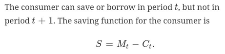
def Problem5():
print("Running problem 5...")
""" part a """
# Define the variables
Ct, Ct1, S = var('ct,ct1,s',real=True)
# Define lambdas
lam1 = symbols('lambda1',real = True)
lam2 = symbols('lambda2', real=True)
# Define r
r = 0.1
# Define the objective function. NOTE: We set the objctive as negative in order to maixmize
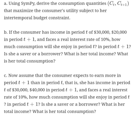
f = (Ct*Ct1)**(1/2)
"""
PART B
"""
print(" *** PART B *** ")
# Define intertemporal budget constraint
Mt = 30000
Mt1 = 20000
const1 = Mt - Mt1 / (1 + r) - Ct - Ct1 / (1 + r)
# Define saving function
const2 = S - Mt + Ct
# Define lagrangian
L = f - lam1 * const1 - lam2 * const2
# Define gradient
gradL = [diff(L, c) for c in [Ct, Ct1, S]]
KKT_eqs = gradL + [const1] + [const2]
sol = solve(KKT_eqs, [Ct,Ct1,S,lam1,lam2],dict=True)[0]
Ctsol = sol[Ct]
Ct1sol = sol[Ct1]
Ssol = sol[S]
print("The consumption at period t is {:.2f}".format(Ctsol))
print("The consumption at period t+1 is {:.2f}".format(Ct1sol))
print("The savings are {:.2f}".format(Ssol))
print("The total income is {:.2f}".format(Mt+Mt1))
print("The toal consumption is {:.2f}".format(Ctsol+Ct1sol))
print()
"""
PART C
"""
print(" *** PART C *** ")
# Define interporal budget constraint
Mt = 30000
Mt1 = 40000
const1 = Mt - Mt1 / (1 + r) - Ct - Ct1 / (1 + r)
# Define saving function
const2 = S - Mt + Ct
# Define lagrangian
L = f - lam1 * const1 - lam2 * const2
# Define gradient
gradL = [diff(L, c) for c in [Ct, Ct1, S]]
KKT_eqs = gradL + [const1] + [const2]
sol = solve(KKT_eqs, [Ct, Ct1, S, lam1, lam2], dict=True)[0]
ctsol = sol[Ct]
Ct1sol = sol[Ct1]
Ssol = sol[S]
print("The consumption at period t is {:.2f}".format(Ctsol))
print("The consumption at period t+1 is {:.2f}".format(Ct1sol))
print("The savings are {:.2f}".format(Ssol))
print("The total income is {:.2f}".format(Mt + Mt1))
print("The toal consumption is {:.2f}".format(Ctsol + Ct1sol))
print()
"""
PART D
"""
print(" *** PART D *** ")
# Define interporal budget constraint
Mt = 30000
Mt1 = 30000
const1 = Mt - Mt1 / (1 + r) - Ct - Ct1 / (1 + r)
# Define saving function
const2 = S - Mt + Ct
# Define lagrangian
L = f - lam1 * const1 - lam2 * const2
# Define gradient
gradL = [diff(L, c) for c in [Ct, Ct1, S]]
KKT_eqs = gradL + [const1] + [const2]
sol = solve(KKT_eqs, [Ct, Ct1, S, lam1, lam2], dict=True)[0]
Ctsol = sol[Ct]
; Ct1sol = sol[Ct1]
Ssol = sol[S]
print("The consumption at period t is {:.2f}".format(Ctsol))
print("The consumption at period t+1 is {:.2f}".format(Ct1sol))
print("The savings are {:.2f}".format(Ssol))
print("The total income is {:.2f}".format(Mt + Mt1))
print("The toal consumption is {:.2f}".format(Ctsol + Ct1sol))
print()
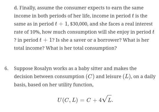
def Problem6():
print("Running problem 6...")
# Define parameters
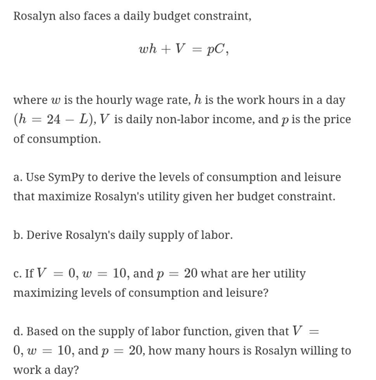
w = 10
V = 0
p = 20
# Define variables
C, L = var('C,L', real=True)
# Define lambda
lam = symbols('lambda', real=True)
# Define objective
f = (C + 4*L**(1/2)) # Negative so we maximize it
# Define the budget constraint
constraint1 = w*(24 - L) + V - p*C
# Define lagrangian
Lag = f - lam * constraint1
# Define gradient
gradL = [diff(Lag, c) for c in [C, L]]
KKT_eqs = gradL + [constraint1]
sol = solve(KKT_eqs, [C, L, lam], dict=True)[0]
#print(sol)
Csol = sol[C]
Lsol = sol[L]
fval = f.subs(C, Csol)
fval = fval.subs(L, Lsol)
""" Part b """
print("The consumption is {:.2f} and the leisure is {:.2f}".format(Csol, Lsol))
""" Part c """
print("The utility is {:.2f}".format(fval))
""" Part d """
print("Rosalyn is willing to work {:.0f} hours a day".format(24 - Lsol))
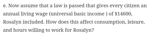
""" Part e """
# For this case, V = 14600/365
V = 14600/365
# We compute all variables again
constraint1 = w * (24 - L) + V - p * C
p; # Define lagrangian
Lag = f - lam * constraint1
# Define gradient
gradL = [diff(Lag, c) for c in [C, L]]
KKT_eqs = gradL + [constraint1]
sol = solve(KKT_eqs, [C, L, lam], dict=True)[0]
#print(sol)
Csol = sol[C]
Lsol = sol[L]
fval = f.subs(C, Csol)
fval = fval.subs(L, Lsol)
print("With the new law, Rosalyn is willing to work {:.0f} hours a day and her utility is {:.2f}".format(24 - Lsol, fval))
if __name__ == '__main__':
Problem1()
Problem2()
Problem3()
Problem4()
Problem5()
Problem6()