Python Program to Implement Model Fitting Assignment Solution.

!pip install otter-grader

# Initialize Otter

import otter

grader = otter.Notebook("lab8.ipynb")

# Lab 8: Fitting Models to Data

In this lab, you will practice using a numerical optimization package `cvxpy` to compute solutions to optimization problems. The example we will use is a linear fit and a quadratic fit.

import pandas as pd

import numpy as np

%matplotlib inline

import matplotlib.pyplot as plt

import seaborn as sns

## Objectives for Lab 8:

Models and fitting models to data is a common task in data science. In this lab, you will practice fitting models to data. The models you will fit are:

* Linear fit

* Normal distribution

## Boston Housing Dataset

from sklearn.datasets import load_boston

boston_dataset = load_boston()

print(boston_dataset['DESCR'])

housing = pd.DataFrame(boston_dataset['data'], columns=boston_dataset['feature_names'])

housing['MEDV'] = boston_dataset['target']

housing.head()

fig, ax = plt.subplots(figsize=(10, 7))

sns.scatterplot(x='LSTAT', y='MEDV', data=housing)

plt.show()

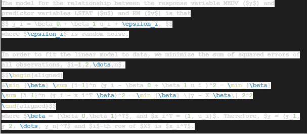
The model for the relationship between the response variable MEDV ($y$) and predictor variables LSTAT ($u$) and RM ($v$) is that

$$ y_i = \beta_0 + \beta_1 u_i + \epsilon_i, $$

where $\epsilon_i$ is random noise.

In order to fit the linear model to data, we minimize the sum of squared errors of all observations, $i=1,2,\dots,n$.

$$\begin{aligned}

&\min_{\beta} \sum_{i=1}^n (y_i - \beta_0 + \beta_1 u_i )^2 = \min_{\beta} \sum_{i=1}^n (y_i - x_i^T \beta)^2 = \min_{\beta} \|y - X \beta\|_2^2

\end{aligned}$$

where $\beta = (\beta_0,\beta_1)^T$, and $x_i^T = (1, u_i)$. Therefore, $y = (y_1, y_2, \dots, y_n)^T$ and $i$-th row of $X$ is $x_i^T$.

## Question 1: Constructing Data Variables

Define $y$ and $X$ from `housing` data.

y = housing['MEDV']

X1 = housing['LSTAT'].to_frame()

X1.insert(0, 'intercept', np.ones((len(y),1)))

#X.insert(0, 'intercept', X1)

grader.check("q1")

## Installing CVXPY

First, install `cvxpy` package by running the following bash command:

!pip install cvxpy

## Question 2: Fitting Linear Model to Data

Read this example of how cvxpy problem is setup and solved: https://www.cvxpy.org/examples/basic/least_squares.html

The usage of cvxpy parallels our conceptual understanding of components in an optimization problem:

* `beta` are the variables $\beta$

* `loss` is sum of squared errors

* `prob` minimizes the loss by choosing $\beta$

Make sure to extract the data array of data frames (or series) by using `values`: e.g., `X.values`

beta2

import cvxpy as cp

beta2 = cp.Variable(2)

loss2 = cp.sum_squares(y.values-X1.values @ beta2)

prob2 = cp.Problem(cp.Minimize(loss2))

prob2.solve()

yhat2 = X1.values@beta2.value

grader.check("q2")

## Question 3: Visualizing resulting Linear Fit

Visualize fitted model by plotting `LSTAT` by `MEDV`.

fig, ax = plt.subplots(figsize=(10, 7))

sns.scatterplot(x='LSTAT', y='MEDV', data=housing, ax = ax, label='Data')

sns.scatterplot(housing['LSTAT'], yhat2, label='Fit', ax = ax)

plt.legend()

plt.show()

## Question 4: Fitting Quadratic Model to Data

Add a column of squared `LSTAT` values to `X`. The new model is,

Then, fit a quadratic model to data.

X2 = X1.copy()

X2.insert(2, 'LSTAT^2', X2['LSTAT']**2)

beta4 = cp.Variable(3)

loss4 = cp.sum_squares(y.values-X2.values @ beta4)

prob4 = cp.Problem(cp.Minimize(loss4))

prob4.solve()

yhat4 = X2.values@beta4.value

grader.check("q4a")

Visualize quadratic fit:

fig, ax = plt.subplots(figsize=(10, 7))

sns.scatterplot(x='LSTAT', y='MEDV', data=housing, ax = ax, label='Data')

sns.scatterplot(housing['LSTAT'], yhat4, label='Fit', ax = ax)

plt.legend()

plt.show()

---

To double-check your work, the cell below will rerun all of the autograder tests.

grader.check_all()

## Submission

Make sure you have run all cells in your notebook in order before running the cell below, so that all images/graphs appear in the output. The cell below will generate a zip file for you to submit. **Please save before exporting!**

# Save your notebook first, then run this cell to export your submission.

grader.export()