Instructions
Requirements and Specifications


Source Code
% EE 7330 Modern Radar Theory
% Spring 2022 - Project 00
% Team 5
% Trevor Scarberry, Matthew Scharf, Siddhant Sharma
clc
clear all
close all
%% Parameters
%variables
Ptx = 150e3;
Fc = 9.4e9;
tau = 1.2e-6;
PRF = 2e3;
PRI = 1/PRF;
Gtx_dB = 45.25;
Tdw = 18.3e-3;
F0_dB = 2.5;
Ltx_dB = 3.1;
Lrx_dB = 2.4;
Lsp_dB = 3.2;
RT_km = 5:105;
RT = RT_km*1000;
Latm_dB = .16*2*RT_km;
sigma1_dB = 0;
sigma2_dB = -10;
SNRM_dB = 12;
% vT = [150 250 400] * 0.5144447;
vT = [150 250 400];
c = 3e8;
kB = 1.38e-23;
T = 290;
B = 1/tau;
lambda = c/Fc;
Rtgt_km = [25 50 70]; %target ranges, km
Rtgt = Rtgt_km * 1000;
Vtgt = [-15, 5, -10]; %Target velocities, m/s
%convert dB to abs
Gtx = 10^(Gtx_dB/10);
F0 = 10^(F0_dB/10);
Ltx = 10^(Ltx_dB/10);
Lrx = 10^(Lrx_dB/10);
Lsp =10^(Lsp_dB/10);
Latm = 10.^(Latm_dB/10);
SNRM = 10^(SNRM_dB/10);
sigma1 = 10^(sigma1_dB/10);
sigma2 = 10^(sigma2_dB/10);
np = floor(Tdw * PRF);
M = np;
L = Ltx*Lrx*Lsp.*(Latm);
N = kB*B*T*F0;
SNR_M_arr_dB = ones(1,length(RT)) * SNRM_dB; % Need array to plot
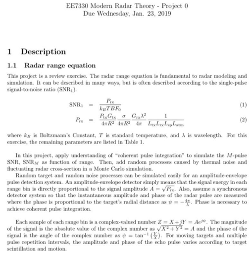
%% 1.a reproduce curves for SNRM versus range
Prx = (Ptx*Gtx^2*lambda^2)./((RT).^4*(4*pi)^3.*L); % here we calculate prc according to equation (2), but without the standard deviations
SNR0 = Prx./N;
% Here we complete the calculations of Prx and SNR for each standard
% deviation (positive and negative)
Prx1 = Prx*sigma1;
SNR1 = M*Prx1/(N);
Prx2 = Prx*sigma2;
SNR2 = M*Prx2/(N);
figure;
plot(RT_km, 10*log10(SNR1), '-b', 'LineWidth', 2);
hold on;
plot(RT_km, 10*log10(SNR2),'-k', 'LineWidth', 2);
hold on;
plot(RT_km, SNR_M_arr_dB,'r--', 'LineWidth', 2);
ylabel('SNR (dB)');
xlabel('Range (km)');
title('SNR vs Range')
legend('\sigma_1 = 0 dBsm ', '\sigma_2 = -10 dBsm','Threshold');
grid on;
xlim([min(RT_km) max(RT_km)]);
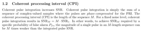
%% 1.b monte carlo sim
% we simulate 1000 events of randomness
for n = 1:1000
RCS1 = random('exp',sigma1,[M 1]);
RCS2 = random('exp',sigma2+1,[M 1]);
y1a(n,:) = sum(RCS1)*SNR1/M;
y2a(n,:) = sum(RCS2)*SNR2/M;
end
%obtain mean and standard deviation
y1avg = mean(y1a,1);
y1std = std(y1a,1,1);
y2avg = mean(y2a,1);
y2std = std(y2a,1,1);
%convert to db, create data for plots
y1avg_dB = 10*log10(y1avg);
y1avg_plus_std = 10*log10(y1avg+y1std);
y1avg_minus_std = 10*log10(y1avg-y1std);
y2avg_dB = 10*log10(y2avg);
y2avg_plus_std = 10*log10(y2avg+y2std);
y2avg_minus_std = 10*log10(y2avg-y2std);
%plot
figure;
hold on;
plot(RT_km,y1avg_dB)
plot(RT_km,y1avg_plus_std)
plot(RT_km,y1avg_minus_std)
plot(RT_km, SNR_M_arr_dB,'r--', 'LineWidth', 2);
plot(RT_km,y2avg_dB)
plot(RT_km,y2avg_plus_std)
plot(RT_km,y2avg_minus_std)
xlabel('Range[km]')
ylabel('SNR[dB]')
title('SNR vs Range (n=1000)')
legend('\sigma_1 = 0 dBsm ', '\sigma_2 = -10 dBsm','Threshold');
grid on;
xlim([min(RT_km) max(RT_km)]);
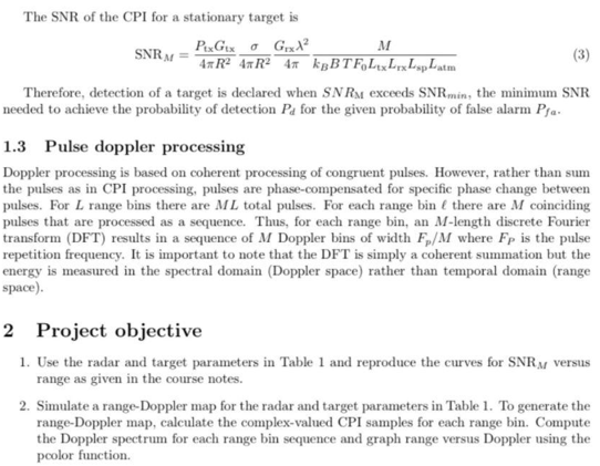
%% Part 2 - Range-Doppler Map
% here we calculate the signal amplitudes according toi equation (17.2) on
% the book
A = sqrt(Prx1);
% The next 3 lines calculates the amplitudes at each of the desired
% locations inside the range of study
A1= sqrt((Ptx*Gtx^2*sigma1*lambda^2)./((Rtgt(1))^4*(4*pi)^3.*L));
A2= sqrt((Ptx*Gtx^2*sigma1*lambda^2)./((Rtgt(2))^4*(4*pi)^3.*L));
A3= sqrt((Ptx*Gtx^2*sigma1*lambda^2)./((Rtgt(3))^4*(4*pi)^3.*L));
% The next line calculates the transmited frequency according to equation
% (17.1) on the book
Fd = 2*Vtgt/lambda;
%resolution = 1/(PRI*M);
% y1 = complex(zeros(length(RT_km),M));
% y2 = complex(zeros(length(RT_km),M));
% y3 = complex(zeros(length(RT_km),M));
%
% for l = 1:length(RT_km)
% for m = 1:M
%
% y1(l,m) = A(l)*exp(-1i*4*pi*Rtgt(1)/lambda)*exp(1i*2*pi*m*PRI*Fd(1));
% y2(l,m) = A(l)*exp(-1i*4*pi*Rtgt(2)/lambda)*exp(1i*2*pi*m*PRI*Fd(2));
% y3(l,m) = A(l)*exp(-1i*4*pi*Rtgt(3)/lambda)*exp(1i*2*pi*m*PRI*Fd(3));
% end
% end
% y0 = y1+y2+y3;
% Y =fftshift(fft(y0,[],2));
% Y1 = fftshift(fft(y1,[],2));
% Y2 = fftshift(fft(y2,[],2));
% Y3 = fftshift(fft(y3,[],2));
% We create the pulse-Doppler data matrix filled with zeros
y1 = complex(zeros(length(RT_km),M));
% Now, for every bin l0 and for every bin on the range M, we calculate
% the spatial Doppler signal
for l = 1:length(Rtgt_km)
for m = 1:M
idx = find(RT_km==Rtgt_km(l)); % One of the problems were here. The variable y1 has the same number
% of rows as elements in the vector
% RT_km, so when the values were
% changed for every value in
% Rtgt_km, the indices used were
% wrong
y1(idx,m) = A1(l)*exp(-1i*4*pi*Rtgt_km(l)/lambda)*exp(1i*2*pi*m*PRI*Fd(l));
end
end
% Now, we apply the fast fourier transform to the matrix and we obtain a
% complex number X + jY
Y1 = fftshift(fft(y1, [], 2), 2); % Another fix was done here. The fftshift and fft
% functions were called with
% incorrect arguments for number of
% dimensions
% Y2 = fftshift(fft(y2,[],2));
% Y3 = fftshift(fft(y3,[],2));
% Here we define the range of frequencies (x) and the space (y)
x = linspace((-PRF/2),(PRF/2),M);
y = linspace(min(RT_km),max(RT_km),length(RT_km));
%
% %plots
% figure
% hold on
% subplot(1,3,1)
% pcolor(x,y,abs((Y1)))
% title('range-doppler plot v = 150')
% xlabel('Doppler Freq (Hz)')
% ylabel('range(km)')
% shading interp
% colormap jet
% colorbar;
% subplot(1,3,2)
% pcolor(x,y,abs((Y2)))
% title('range-doppler plot v = 250')
% xlabel('Doppler Freq (Hz)')
% ylabel('range(km)')
% shading interp
% colormap jet
% colorbar;
% subplot(1,3,3)
% pcolor(x,y,abs((Y3)))
% title('range-doppler plot v = 400')
% xlabel('Doppler Freq (Hz)')
% ylabel('range(km)')
% shading interp
% colormap jet
% colorbar;
figure
hold on
pcolor(x,y,abs(Y1))
title('range-doppler plot')
xlabel('Doppler Freq (Hz)')
ylabel('range(km)')
xlim([-PRF/2,PRF/2]);
ylim([min(RT_km), max(RT_km)]);
shading interp
colormap jet
colorbar;
% figure;
% subplot(3,1,1)
% plot(x,abs(Y1))
% xlabel("Doppler Freq (Hz)");
% ylabel("Range (km)");
% % xlim([min(RT_km), max(RT_km)]);
% grid on;
% subplot(3,1,2)
% plot(x,abs(Y2))
% xlabel("Doppler Freq (Hz)");
% ylabel("Range (km)");
% % xlim([min(RT_km), max(RT_km)]);
% grid on;
% subplot(3,1,3)
% plot(x,abs(Y3))
% xlabel("Doppler Freq (Hz)");
% ylabel("Range (km)");
% % xlim([min(RT_km), max(RT_km)]);
% grid on;