Instructions
Requirements and Specifications
Source Code
# Initialize Otter
import otter
grader = otter.Notebook("lab3-visualization.ipynb")
import pandas as pd
import numpy as np
import altair as alt
# Assignment: Data visualization
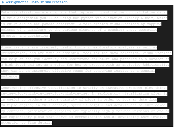
Data visualizations are graphics that represent quantitative or qualitative data. In this assignment you'll be using the python visualization library Altair, which is built around the pandas dataframe. Altair creates visualizations by mapping columns of a dataframe to the various elements of a graphic: axes, geometric objects, and aesthetics.
Visualizations are immensely useful tools in exploratory analysis as well as presentation, and are thus an essential tool for the data scientist. Visualizations can help an analyst identify and understand structure and patterns in a dataset at a high level and act as a guide for how to proceed with an analysis. Additionally, they can be an extremely effective means for conveying results to a general audience.
Constructing effective visualization is usually an iterative process: plot-think-revise-plot-think-revise-plot-think-revise. In exploratory visualization often it is useful to produce a large quantity of plots in order to look at data from multiple angles; in this context, speed is helpful and details can be overlooked. By contrast, presentation graphics are typically highly refined versions of one or two exploratory plots that serve as communication tools; developing them involves attention to fine detail.
---
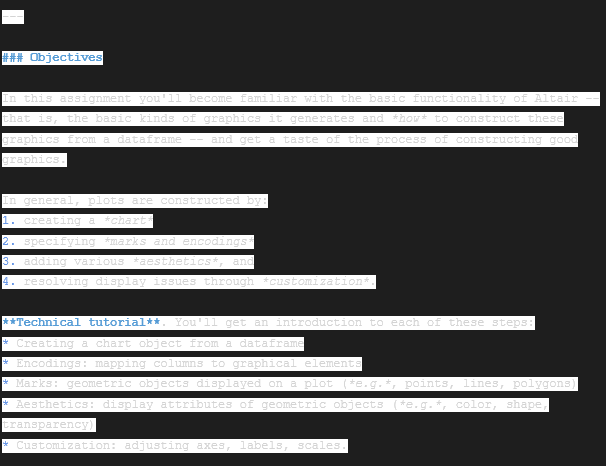
### Objectives
In this assignment you'll become familiar with the basic functionality of Altair -- that is, the basic kinds of graphics it generates and *how* to construct these graphics from a dataframe -- and get a taste of the process of constructing good graphics.
In general, plots are constructed by:
1. creating a *chart*
2. specifying *marks and encodings*
3. adding various *aesthetics*, and
4. resolving display issues through *customization*.
**Technical tutorial**. You'll get an introduction to each of these steps:
* Creating a chart object from a dataframe
* Encodings: mapping columns to graphical elements
* Marks: geometric objects displayed on a plot (*e.g.*, points, lines, polygons)
* Aesthetics: display attributes of geometric objects (*e.g.*, color, shape, transparency)
* Customization: adjusting axes, labels, scales.
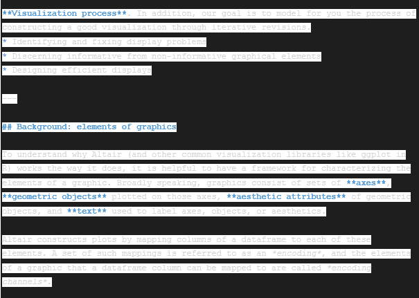
**Visualization process**. In addition, our goal is to model for you the process of constructing a good visualization through iterative revisions.
* Identifying and fixing display problems
* Discerning informative from non-informative graphical elements
* Designing efficient displays
---
## Background: elements of graphics
To understand why Altair (and other common visualization libraries like ggplot in R) works the way it does, it is helpful to have a framework for characterizing the elements of a graphic. Broadly speaking, graphics consist of sets of **axes**, **geometric objects** plotted on those axes, **aesthetic attributes** of geometric objects, and **text** used to label axes, objects, or aesthetics.
Altair constructs plots by mapping columns of a dataframe to each of these elements. A set of such mappings is referred to as an *encoding*, and the elements of a graphic that a dataframe column can be mapped to are called *encoding channels*.
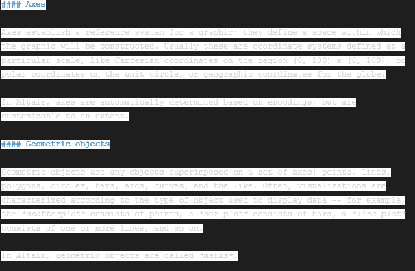
#### Axes
Axes establish a reference system for a graphic: they define a space within which the graphic will be constructed. Usually these are coordinate systems defined at a particular scale, like Cartesian coordinates on the region (0, 100) x (0, 100), or polar coordinates on the unit circle, or geographic coordinates for the globe.
In Altair, axes are automatically determined based on encodings, but are customizable to an extent.
#### Geometric objects
Geometric objects are any objects superimposed on a set of axes: points, lines, polygons, circles, bars, arcs, curves, and the like. Often, visualizations are characterized according to the type of object used to display data -- for example, the *scatterplot* consists of points, a *bar plot* consists of bars, a *line plot* consists of one or more lines, and so on.
In Altair, geometric objects are called *marks*.
#### Aesthetic attributes
The word 'aesthetics' is used in a variety of ways in relation to graphics; you will see this in your reading. For us, 'aesthetic attirbutes' will refer to attributes of geometric objects like color. The primary aesthetics in statistical graphics are color, opacity, shape, and size.
In Altair, aesthetic attributes are called *mark properties*.
#### Text
Text is used in graphics to label axes, geometric objects, and legends for aesthetic mappings. Text specification is usually a step in customization for presentation graphics, but often skipped in exploratory graphics. Carefully chosen text is very important in this context, because it provides essential information that a general reader needs to interpret a plot.
In Altair, text is usually controlled as part of encoding specification.
---
## 0. Dataset: GDP and life expectancy
We'll be illustrating Altair functionality and visualization process using a dataset comprising observations of life expectancies at birth for men, women, and the general population, along with GDP per capita and total population for 158 countries at approximately five-year intervals from 2000 to 2019.
* Observational units: countries.
* Variables: country, year, life expectancy at birth (men, women, overall), GDP per capita, total population, region (continent), and subregion.
The data come from merging several smaller datasets, mostly collected from [World Bank Open Data](https://data.worldbank.org/). The result is essentially a convenience sample, but descriptive analyses without inference are nonetheless interesting and suggestive.
Your focus won't be on acquainting yourself with the data carefully or on tidying. The cell below imports and merges component datasets.
# import and format country regional information
countryinfo = pd.read_csv(
'data/country-info.csv'
).iloc[:, [2, 5, 6]].rename(
columns = {'alpha-3': 'Country Code'}
)
# import and format gdp per capita
gdp = pd.read_csv(
'data/gdp-per-capita.csv', encoding = 'latin1'
).drop(columns = ['Indicator Name', 'Indicator Code']).melt(
id_vars = ['Country Name', 'Country Code'],
var_name = 'Year',
value_name = 'GDP per capita'
).astype({'Year': 'int64'})
# import and format life expectancies
life = pd.read_csv(
'data/life-expectancy.csv'
).rename(columns={'All': 'Life Expectancy',
'Male': 'Male Life Expectancy',
'Female': 'Female Life Expectancy'
})
# import population data
pop = pd.read_csv(
'data/population.csv', encoding = 'latin1'
).melt(
id_vars = ['Country Name', 'Country Code'],
var_name = 'Year',
; value_name = 'Population'
).astype({'Year': 'int64'}).drop(columns = 'Country Name')
# merge
merge1 = pd.merge(life, gdp, how = 'left', on = ['Country Name', 'Year'])
merge2 = pd.merge(merge1, countryinfo, how = 'left', on = ['Country Code'])
merge3 = pd.merge(merge2, pop, how = 'left', on = ['Country Code', 'Year'])
# final data
data = merge3.dropna().drop(
columns = 'Country Code'
)
data.head()
## 1. A starting point: scatterplot of life expectancy against GDP per capita
Here you'll see how marks and encodings work in a basic sense, along with some examples of how to adjust encodings.
The following cell constructs a scatterplot of life expectancy at birth against GDP per capita; each point corresponds to one country in one year. The syntax works as follows:
* `alt.Chart()` begins by constructing a 'chart' object constructed from the dataframe;
* the result is passed to `.mark_circle()`, which specifies a geometric object (circles) to add to the chart;
* the result is passed to `.encode()`, which specifies which columns should be used to determine the coordinates of the circles.
# basic scatterplot
alt.Chart(data).mark_circle().encode(
x = 'GDP per capita',
y = 'Life Expectancy'
)
### Question 1ai. Different marks
The cell below is a copy of the previous cell. Have a look at the [documentation on marks](https://altair-viz.github.io/user_guide/marks.html) for a list of the possible mark types. Try out a few alternatives to see what they look like! Once you're satisfied, change the mark to points.
# basic scatterplot
alt.Chart(data).mark_circle().encode( # your turn here
x = 'GDP per capita',
y = 'Life Expectancy'
)
### Question 1aii.
What is the difference between points and circles, according to the documentation?
_Type your answer here, replacing this text._
### Axis adjustments with `alt.X()` and `alt.Y()`
An initial problem that would be good to resolve before continuing is that the y axis label isn't informative. Let's change that by wrapping the column to encode in `alt.Y()` and specifying the title manually.
# change axis label
alt.Chart(data).mark_circle().encode(
x = 'GDP per capita',
y = alt.Y('Life Expectancy', title = 'Life Expectancy at Birth')
)
`alt.Y()` and `alt.X()` are helper functions that modify encoding specifications. The cell below adjusts the scale of the y axis as well; since above there are no life expectancies below 30, starting the y axis at 0 adds whitespace.
# don't start y axis at zero
alt.Chart(data).mark_circle().encode(
x = 'GDP per capita',
y = alt.Y('Life Expectancy', title = 'Life Expectancy at Birth', scale = alt.Scale(zero = False))
)
In the plot above, there are a lot of points squished together near $x = 0$. It will make it easier to see the pattern of scatter in that region to adjust the x axis so that values are not displayed on a linear scale. Using `alt.Scale()` allows for efficient axis rescaling; the cell below puts GDP per capita on a log scale.
# log scale for x axis
alt.Chart(data).mark_circle().encode(
x = alt.X('GDP per capita', scale = alt.Scale(type = 'log')),
y = alt.Y('Life Expectancy', title = 'Life Expectancy at Birth', scale = alt.Scale(zero = False))
)
### Question 1b. Changing axis scale
Try a different scale by modifying the `type = ...` argument of `alt.Scale` in the cell below. Look at the [altair documentation](https://altair-viz.github.io/user_guide/generated/core/altair.Scale.html) for a list of the possible types.
# try another axis scale
alt.Chart(data).mark_circle().encode(
x = alt.X('GDP per capita', scale = alt.Scale(type = 'log')), # your turn here
y = alt.Y('Life Expectancy', title = 'Life Expectancy at Birth', scale = alt.Scale(zero = False))
)
---
## 2. Using aesthetic attributes to display other variables
Now that you have a basic plot, you can start experimenting with aesthetic attributes. Here you'll see examples of how to add aesthetics, and how to use them effectively to display information from other variables in the dataset.
Let's start simple. The points are a little too on top of one another. Opacity (or transparency) can be added as an aesthetic to the mark to help visually identify tightly clustered points better. The cell below does this by *specifying a global value for the aesthetic at the mark level*.
# change opacity globally to fixed value
alt.Chart(data).mark_circle(opacity = 0.5).encode(
x = alt.X('GDP per capita', scale = alt.Scale(type = 'log')),
y = alt.Y('Life Expectancy', title = 'Life Expectancy at Birth', scale = alt.Scale(zero = False))
)
If instead of simply modifying an aesthetic, we want to use it to display variable information, we could instead specify the attribute *through an encoding*, as below:
# use opacity as an encoding channel
alt.Chart(data).mark_circle().encode(
x = alt.X('GDP per capita', scale = alt.Scale(type = 'log')),
y = alt.Y('Life Expectancy', title = 'Life Expectancy at Birth', scale = alt.Scale(zero = False)),
opacity = 'Year'
)
Notice that there's not actually any data for 2005. Isn't it odd, then, that the legend includes an opacity value for that year? This is because the variable year is automatically treated as quantitative due to its data type (integer). If we want to instead have a unique value of opacity for each year (*i.e.*, use a discrete scale), we can coerce the data type *within Altair* by putting an `:N` (for nominal) after the column name.
### Question 2a. Data Type Coercing
Map the `Year` column into a nominal data type by putting an `:N` (for nominal) after the column name.
# use opacity as an encoding channel
alt.Chart(data).mark_circle().encode(
x = alt.X('GDP per capita', scale = alt.Scale(type = 'log')),
y = alt.Y('Life Expectancy', title = 'Life Expectancy at Birth', scale = alt.Scale(zero = False)),
; opacity = 'Year' # change made here -- treat year as nominal
)
This displays more recent data in darker shades. Nice, but not especially informative. Let's try encoding year with color instead.
### Question 2b. Color encoding
Map `Year` (as nominal) to color.
# map year to color
...
Pretty, but there's not a clear pattern, so the color aesthetic for year doesn't make the plot any more informative. This **doesn't** mean that year is unimportant; just that color probably isn't the best choice to show year.
Let's try to find a color variable that does add information to the plot. When region is mapped to color, there is a clear(er) pattern consisting of sets of overlapping clusters. This communicates visually that there's some similarity in the relationship between GDP and life-expectancy among countries in the same region.
# map region to color
alt.Chart(data).mark_circle(opacity = 0.5).encode(
x = alt.X('GDP per capita', scale = alt.Scale(type = 'log')),
y = alt.Y('Life Expectancy', title = 'Life Expectancy at Birth', scale = alt.Scale(zero = False)),
color = 'region'
)
That's a little more interesting. Let's add another variable: map population to size, so that points are displayed in proportion to the country's total population.
# map population to size
alt.Chart(data).mark_circle(opacity = 0.5).encode(
x = alt.X('GDP per capita', scale = alt.Scale(type = 'log')),
y = alt.Y('Life Expectancy', title = 'Life Expectancy at Birth', scale = alt.Scale(zero = False)),
color = 'region',
size = 'Population'
)
Great, but highly populous countries in Asia are so much larger than countries in other regions that, when size is displayed on a linear scale, too many data points are hardly visible. Just like the axes were rescaled using `alt.X()` and `alt.Scale()`, other encoding channels can be rescaled, too. Below, size is put on a square root scale.
# rescale size
alt.Chart(data).mark_circle(opacity = 0.5).encode(
x = alt.X('GDP per capita', scale = alt.Scale(type = 'log')),
y = alt.Y('Life Expectancy', title = 'Life Expectancy at Birth', scale = alt.Scale(zero = False)),
color = 'region',
size = alt.Size('Population', scale = alt.Scale(type = 'sqrt')) # change here
)
Not only does this add information, but it makes the regional clusters a little more visible!
## 3. Faceting
Your previous graphic looks pretty good, and is nearly presentation-quality. However, it still doesn't display year information. As a result, each country appears multiple times in the same plot.
*Faceting* is another term for making a panel of plots. This can be used to make separate plots for each year, so that every obeservational unit (country) only appears once on each plot, and possibly an effect of year will be evident.
# facet by year
alt.Chart(data).mark_circle(opacity = 0.5).encode(
x = alt.X('GDP per capita', scale = alt.Scale(type = 'log')),
y = alt.Y('Life Expectancy', title = 'Life Expectancy at Birth', scale = alt.Scale(zero = False)),
color = 'region',
size = alt.Size('Population', scale = alt.Scale(type = 'sqrt'))
).facet(
column = 'Year'
)
### Question 3a. Now each panel is too big.
Resize the individual facets using `.properties(width = ..., height = ...)`. This has to be done *before* faceting. Try a few values before settling on a size that you like.
# resize facets
alt.Chart(data).mark_circle(opacity = 0.5).encode(
x = alt.X('GDP per capita', scale = alt.Scale(type = 'log')),
y = alt.Y('Life Expectancy', title = 'Life Expectancy at Birth', scale = alt.Scale(zero = False)),
color = 'region',
size = alt.Size('Population', scale = alt.Scale(type = 'sqrt'))
).properties(
# your turn here
).facet(
column = 'Year'
)
Looks like life expectancy is increasing over time! Can we also display the life expectancies for each sex separately? To do this, we'll need to rearrange the dataframe a little -- untidy it so that we have one variable that indicates sex, and another that indicates life expectancy.
### Question 3b. Melt for plotting purposes
Drop the `Life Expectancy` column and melt the `Male Life Expectancy`, and `Female Life Expectancy` columns of `data` so that:
* the values appear in a column called `Life Expectancy at Birth`;
* the variable names appear in a column called `Group`.
Store the result as `plot_df` and print the first few rows. It may be helpful to check the [pandas documentation on melt](https://pandas.pydata.org/docs/reference/api/pandas.DataFrame.melt.html?highlight=melt#pandas.DataFrame.melt).
# melt
plot_df = ...
# print first few rows
grader.check("q3_b")
You will need to complete the part above correctly before moving on. The first several rows of `plot_df` should match the following:
plot_df
# check result
pd.read_csv('data/plotdf-check.csv')
Now you can use the `Group` variable you defined to facet by both year and sex. This is shown below:
# facet by both year and sex
alt.Chart(plot_df[plot_df['Group'] != 'Life Expectancy']).mark_circle(opacity = 0.5).encode(
x = alt.X('GDP per capita', scale = alt.Scale(type = 'log')),
y = alt.Y('Life Expectancy at Birth:Q', scale = alt.Scale(zero = False)),
color = 'region',
size = alt.Size('Population', scale = alt.Scale(type = 'sqrt'))
).properties(
width = 250,
height = 250
).facet(
column = 'Year',
row = 'Group'
)
### Question 3c. Adjusting facet layout
It's a little hard to line up the patterns visually between sexes because they are aligned on GDP per capita, not life expectancy -- so we can't really tell without moving our eyes back and forth and checking the axis ticks whether there's much difference in life expectancy rates by sex. Switching the row/column layout gives a better result. Modify the cell below so that facet columns correspond to sex and facet rows correspond to years.
# facet by both year and sex
alt.Chart(plot_df[plot_df['Group'] != 'Life Expectancy']).mark_circle(opacity = 0.5).encode(
x = alt.X('GDP per capita', scale = alt.Scale(type = 'log')),
y = alt.Y('Life Expectancy at Birth:Q', scale = alt.Scale(zero = False)),
color = 'region',
size = alt.Size('Population', scale = alt.Scale(type = 'sqrt'))
).properties(
width = 250,
height = 250
).facet(
column = 'Year', # your turn here
row = 'Group' # your turn here
)
So life expectancy is a bit lower for men on average. But from the plot it's hard to tell if some countries reverse this pattern, since you can't really tell which country is which. Also, the panel is a bit cumbersome. Take a moment to consider how you might improve these issues, and then move on to our suggestion below.
The next parts will modify the dataframe `data` by adding a column. We'll create a copy `data_mod1` of the original dataframe `data` to modify as to not lose track of our previous work:
data_mod1 = data.copy()
### Question 3d. Data transformation and re-plotting
A simple data transformation can help give a clearer and more concise picture of how life expectancy differs by sex. Perform the following steps:
* append a new variable `Difference` to `data_mod1` that gives the difference between female and male (F - M) life expectancies in each country and year;
* modify the your plot in Q3 (b) (general life expectancy against GDP per capita by year) to instead plot the difference in life expectancies at birth against GDP per capita by year.
When modifying the example, be sure to change the axis label appropriately.
# define new variable for difference
data_mod1['Difference'] = ...
# plot difference vs gdp by year
...
"""; #END PROMPT
### Question 3e. Interpretation
Select a graphic for presentation and reproduce it below. State in one sentence why you chose this graphic, and summarize in 1-2 sentences what is shown in the graphic.
# plot here
#### Answer
*Type your answer here.*
## 4. Your turn
Now that you've seen basic functionality of Altair, explore the data further! Construct any plot of your choosing. It does not need to be fancy or elaborate -- this is just an opportunity to work from scratch and play a little while you're primed on plot construction. However, it should be well-sized, appropriately labeled, and visually clean. Some possibilities you could consider are:
* line plots of life expectancy over time based on the dataset `life`;
* scatterplots of life expectancy against population;
* aggregating over year or subregion before plotting.
Please produce a graphic and a brief (1-2 sentence) description of what it shows.
# scratch work here
# final plot
#### Description and Interpretation of Graphic
your description here
---
To double-check your work, the cell below will rerun all of the autograder tests.
grader.check_all()